|
<< Click to Display Table of Contents >> Dynamic Analysis of Belt Conveyors |
  
|
|
<< Click to Display Table of Contents >> Dynamic Analysis of Belt Conveyors |
|
by Mark Alspaugh
Overland Conveyor Co.
In the 5th edition of Belt Conveyors for Bulk Materials published by the engineering committee of the “Conveyor Equipment Manufacturers Association” (and in all previous versions) a subheading in Chapter 6, (Belt Tension, Power, and Drive Engineering) is labeled “Necessary Assumptions”.
As in all engineering investigations of this type, the first question is, “To what degree of accuracy will the computations have to be carried out?” The answer is not simple. Important factors are the overall size, the importance of the installation, and the type and sensitivity of the equipment adjacent to it.
In any case, numerous simplifying assumptions will have to be made to keep the engineering work within reasonable limits. For examples of simplifying assumptions, refer to the problems connected with belt stretch (elastic elongation from accelerating or decelerating forces) and take-up reactions.
During both the acceleration and deceleration cycles, the transient forces imposed result in extra stretch not encountered during steady state operation. This may result in early splice failure, excessive take-up travel, and other difficulties. Calculations (in this book) for acceleration and deceleration treat the system as a rigid body. This is a common practice in the solution of problems in dynamics. And while the results usually are quite satisfactory, there is more cause for concern over the accuracy of results in the case of belt conveyors.
No further attempt will be made to justify simplifying the assumption, because this usually is not of major significance. However, the belt conveyor designer should be aware that, for conveyor systems with very long center belts, stretch considerations should not be overlooked.
Since this was written many years ago, several important considerations have evolved in bulk material handling industries which dictate additional concern for belt elasticity issues.
First, and most importantly, belt conveyance applications have gotten much bigger. When the above paragraphs were written, a typical conveyor might be 36-42” wide carrying 750-1000 tph at velocities of 400 -600 fpm over lengths of 500-1500 ft. It is still true that belt elasticity issues and conveyor dynamics “are not a major issue” on conveyors of this range. And although these conveyors still exist in all industries, many conveyors today are up 72” wide, carrying 5,000-10,000 tph at velocities of 1000-1500 fpm over lengths of 10,000-20,000 ft. And the largest belt conveyors today are up to 120” wide, carrying 40,000 tph at velocities up to 2000 fpm over lengths up to and beyond 50,000 ft. There is no doubt, on these largest applications; simplifying assumptions dealing with belt elasticity are no longer suitable. Ignoring belt elasticity during stopping and starting can have a major impact on the performance of the conveyor.
Secondly, when the above paragraphs were written very few if any conveyor engineers had computers available to do their calculations. Since dynamic problems are computationally difficult, it was absolutely necessary to simplify the analytical process. At that time, it was “common practice in the solution of problems in dynamics” to treat the system as a rigid body. Today, as our computational hardware continues to develop at an extremely rapid pace, engineers are able to treat dynamic problems more accurately.
Third, with computer hardware comes the inevitable availability of engineering software. It is no longer necessary for a belt conveyor engineer to tediously learn and calculate each step in the analytical process as he can simply buy a computational tool and input data as requested. A 1970’s conveyor engineer might have spent weeks pouring over stacks of calculations in order to engineer a 10,000 ft conveyor while a 21st century engineer might only spend minutes evaluating the viability of a 20,000 ft conveyor with a commercially available static analysis software program. Although these programs might provide entirely reliable analysis of a running conveyor, they do little to guide a novice engineer in the proper method of starting and stopping this same machine reliably.
When performing starting and stopping calculations per Chapter 6 (static analysis), it is assumed that all masses are accelerated at the same time, thus assuming the belt is a rigid body and the rotating masses and the belt are rigidly connected (F=Ma). In reality, the torque produced in the motor and transmitted to the belt via the drive pulley creates a stress wave which starts the belt moving gradually as the wave propagates along the belt. Stress variations along the belt (and therefore elastic stretch of the belt) are caused by these longitudinal waves dampened by internal friction in the belt and material and resistance to motion.
Many publications since 1959 have documented that neglecting belt elasticity in high capacity and/or long length conveyors during stopping and starting can lead to incorrect selection of the belting, drive and take-up device. Failure to include transient response to elasticity can result in inaccurate prediction of:
1- Maximum belt stresses and therefore belt strength safety factors (particularly in the splice)
2- Maximum forces on pulleys
3- Minimum belt stresses and therefore material spillage, belt or idler damage
4- Take-up force requirements
5- Take-up travel and speed requirements
6- Drive slip
7- Breakaway torque
8- Holdback torque
9- Load sharing between multiple drives
10- Material stability on an incline
It is therefore important a mathematical model of the belt conveyor that can take belt elasticity into account during stopping and starting be considered in some applications. As these techniques are perfected, they will become part of the design process in all belt conveyors.
The components of the conveyor that have the most affect on starting and stopping are:
1- Motor (or Brake)
2- Coupling (Torque transmission device)
3- Drive Pulley
4- Belting (elasticity)
5- Idlers (and all resistance to belt motion)
6- Take-up
The general mathematical model should contain mathematical expressions describing each of these components and the relationships between them.
By far, the most difficult component to model is the belt itself. Many methods of analyzing a belt’s physical behavior have been studied and various techniques have been used. The most commonly used method today is a viscoelastic rheological model.
Viscoelasticity is the property of materials that exhibit both viscous and elastic characteristics when undergoing deformation. Viscous materials, like honey, resist shear flow and strain linearly with time when a stress is applied. Elastic materials strain instantaneously when stretched and just as quickly return to their original state once the stress is removed. Viscoelastic materials have elements of both of these properties and, as such, exhibit time dependent strain. Whereas elasticity is usually the result of bond stretching along crystallographic planes in an ordered solid, viscoelasticity is the result of the diffusion of atoms or molecules inside of an amorphous material.
A few of the many types of viscoelastic models which used to describe the dynamic properties of belts include:
a) Elastic Solid
b) Elastic Solid with Coulomb Friction
c) Kelvin Solid
d) Three-Parameter Standard Solid
Other four and five parameter models have been submitted to the industry for consideration. No attempt will be made to support one model over another in this discussion. However, an appropriate model needs to address:
1- Elastic modulus of the belt longitudinal tensile member
2- Resistances to motion which are velocity dependent (i.e. idlers)
3- Viscoelastic losses due to rubber-idler indentation
4- Apparent belt modulus changes due to belt sag between idlers
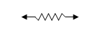
Finite element method (FEM) is a powerful technique originally developed for numerical solution of complex problems in structural mechanics, and it remains the method of choice for complex systems. In the FEM, the structural system is modeled by a set of appropriate finite elements interconnected at points called nodes. Elements may have physical properties such as mass and rheological spring as illustrated in Figure 1.
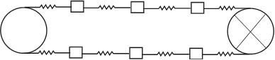
Figure 1
The elements are interconnected only at the exterior nodes, and altogether they should cover the entire domain as accurately as possible. Nodes will have nodal (vector) displacements or degrees of freedom which may include translations, rotations, and for special applications, higher order derivatives of displacements. Whereas elements representing intermediate section of belt and idlers may only have simple displacements, elements representing a take-up device are much more complicated to represent gravity or other mechanical subsystems. When the nodes displace, they will drag the elements along in a certain manner dictated by the element formulation. In other words, displacements of any points in the element will be interpolated from the nodal displacements, and this is the main reason for the approximate nature of the solution.
Hooke's law, which states that force is a linear function of displacement, forms the basis of classical stress analysis, and thus, of modern finite element stress analysis. In finite element analysis, the matrix equation {F} = [K]{U} is solved for the displacement vector, {U}, from the force vector, {F} and the stiffness matrix, [K]. Subsequently, the stresses are calculated from the equation {s}=E{e}, where {e} is the strain vector, which is a normalized displacement vector. E is Young's modulus that corresponds to Hooke's constant, k. This method works well if the analyzed system is always at rest or in a steady state. We consider a belt conveyor running at a constant speed to be in a steady or static state (not contracting or expanding). However, in practical mechanical or structural engineering, the static case should never dictate the final design. The design must always consider the "worst case scenario," which generally occurs when the system is not at steady state, when the forces, and thus the stresses, are greater or less than those under static conditions. In a belt conveyor, this occurs during starting and stopping when the belt is expanding or contracting. A unique characteristic of belt conveyors as the belt is supported on spaced idlers, is low stresses can be just as bad as high stresses.
Once the problem has been discretized, the next step is to determine the matrices which represent it, starting with the elementary matrices. The elementary mass matrix is given by
![]()
The elementary stiffness matrix is calculated by using:
![]()
Finally, the elementary damping matrix is obtained from the stiffness and mass matrices (see below).
The assembly of the global matrices leads to the system equation:
![]()
Where [M], [C], [K] are the global mass, damping and stiffness matrices respectively and {F(t)} the load vector. {}, {}, {} are global accelerations, velocities and displacement vectors respectively.
Mass and stiffness matrices are rather straightforward, however damping, despite its importance, is rather difficult to determine. Viscoelastic phenomena associated with the matrix and the internal slipping of bulk materials are main sources of internal damping of a belt conveyor. These sources are quite difficult to be evaluated, yielding to deviations of the numeric results.
Characterization of damping forces in a vibrating structure has long been an active area of research in structural dynamics. Despite significant research, however, a thorough understanding of damping mechanism has not been attained. A major reason for this is that the state variables that govern damping forces are generally not as clear as they are for inertia and stiffness forces. There are advanced research results to identify a general model of damping (Adhikari, 2000) or the estimation of damping in a random vibrating system (Rudinger, 2002). However, the most common approach is to use viscous damping or Rayleigh damping, in which it is assumed that the damping matrix is proportional to the mass [M] and stiffness matrices [K], or:
[1] ![]()
For large systems, identification of valid damping coefficients and ß for all significant modes is a very complicated task. This assumption has no physical basis but it is mathematically convenient to approximate low damping in this way when exact damping values are not known. The dividing line between under damped and over damped systems where the equation of motion has a damping value that is equal to the critical damping.
How to Incorporate Damping into Belt Conveyor Dynamic Analysis?
Since belt conveyor dynamic analysis starts with the steady state condition of running and ends with the same steady state running condition (stop and restart), an under damped or over damped system will return to a lower or higher steady state energy condition (power requirement). Therefore, the analysis itself can be used to “tune” damping (i.e. increase or decrease in order to return to the original energy state).
Keep in mind, this “tuning” procedure is based on the assumption the initial power requirements of the machine and analysis condition is accurate within reason. This assumption can be confirmed by actual data collection if the machine is built. If not, the best power prediction should be used before commonly added safety margins are used to select components.
Any analysis must begin with initial conditions (t=0). The assumed initial condition of this analysis comes from the steady-state running condition (static analysis) as described in Chapter 6. Since this initial condition is based on running at full speed, the first part of dynamic analysis must simulate the transient condition of stopping.
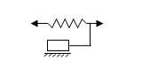
Lumped masses are derived from material weight, belt weight, pulleys, etc. The composite rheological spring element is derived from the selected belt carcass and rubber covers properties and calculated resistances to motion as developed previously. Elements are initially displaced to equal the calculated running stress (F(t) in each element as illustrated in Figure 2.
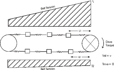
Figure 2
The difference between T1 (tight side drive tension) and T2 (slack side drive tension) in the belt equals the torque across the drive pulley while running which matches the torque applied by the drive. In this steady-state condition, the velocities around the conveyor at each element are close to constant.
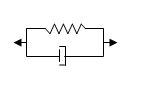
Figure 3 represents a time (dt) shortly after the drive torque is removed to simulate a free drift stop.
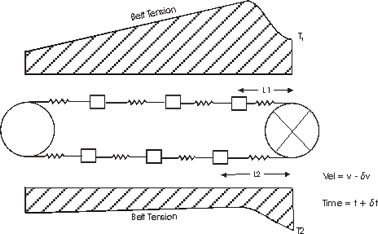
Figure 3
The sequence of events that follow are:
1- The removal of drive torque, leaves the effective tension across the pulley (T1 - T2) unbalanced causing a rapid deceleration of the drive pulley.
2- The velocity differential causes a shortening of the spring preceding the pulley and a lengthening of the spring past the pulley. The other spring lengths stay the same.
3- The change in the spring length causes a tension decrease between the pulley and proceeding mass and tension increase between the pulley and the next mass.
4- The change in tension on one side of these masses causes a force imbalance on that mass and it begins to decelerate causing the force imbalance to propagate to the next mass.
The result is a wave of decreasing tension propagating down the carry side of the conveyor and a wave of increasing tension propagating down the return side. These are often referred to as tension and compression waves.
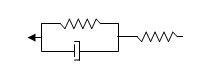
In Figure 4, a gravity take-up pulley is added immediately past the drive pulley and the same scenario is modeled. Now the tension increase in the next element creates a force imbalance on the take-up pulley causing it to accelerate upwards. Since the take-up absorbs the tension increase, the return belt past the take-up is not affected by the drive torque loss until the “compression” wave propagates completely around the conveyor.
If a brake is applied to the drive pulley to stop the conveyor faster, a greater tension imbalance is created causing a faster velocity decrease and decreased stopping time. And of course, the resulting tension and compression waves will be larger.
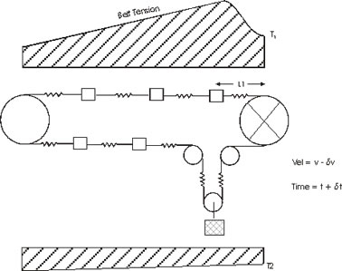
Figure 4
Whether drifting to a stop or applying a braking torque, all belt velocities will eventually reach zero and the entire belt will be at rest (v=0). These stopped conditions are then saved and used as the initial conditions for the next phase of the dynamic process: starting.
The exact same rheological elements and lumped masses are used during the restart. The only difference is now a mathematical model of the drive train during its acceleration phase must be developed and applied to the drive pulley. And there are many types of drive types and starting algorithms to consider.
1- Across-the-line AC Motors
2- Wound Rotor Motors with Resistor Step Starting
3- Reduced Voltage Solid State SCR
4- Constant Fill Fluid Couplings
5- Variable Fill Fluid Couplings
6- Hydro viscous Clutch
7- DC Motors
8- Variable Frequency AC Drives
A direct coupled across-the-line start requires the characteristic speed-torque curve of the motor to be applied to the drive pulley. All other drive types require the adjustment of the motor characteristic torque according to the appropriate ancillary equipment.
All drive types can be placed in one of two categories; torque limiting or time limiting. An example of a torque limiting device is a constant fill fluid coupling. The geometry of the coupling, fill media and fill volume will dictate how much torque is applied to the conveyor belt. With this type drive, variations in total driven mass (different loads) will result in different acceleration times. A time limiting device such as a variable fill fluid coupling, can output a variable torque depending on a feedback mechanism. A preset acceleration velocity curve can be set and maintained no matter how much mass is being accelerated.
Since dynamic analysis as described above is still a very complex mathematical process, it is not used nor required on all belt conveyors. The question that was asked in the first edition of this book in the 1960’s must still be asked; “To what degree of accuracy will the computations have to be carried out?”
The difference is in the 1960’s only a few academics were addressing dynamic issues and the cost of access was prohibitive for the practicing engineer if available at all. Today, there are advanced dynamic analysis programs used by many companies and any conveyor can be a candidate for dynamic review. However, there still is a cost associated with advanced simulation and therefore the question of when this analysis is required is still asked. The answer is still difficult to answer and often still based on the cost of the equipment and significance of the conveyor to the mine or plant. The higher the equipment cost and the more important the conveyor, the more likely the added insurance of upfront analysis is spent.
In an attempt to provide some better, more concrete guidelines, the following lists have been developed.
Common problems on existing conveyors often identified by dynamic analysis
1- Premature belt splice failures
2- Belt breaks other than at splices
3- Repetitive pulley failures
4- Excessive take-up travel
5- Take-up component failures (ropes, sheaves, etc)
6- Drive slip
7- Concave vertical curve liftoff during starting or stopping
8- Brake failures
New Applications requiring dynamic analysis to insure proper design
1- Long lengths (greater than 1 mile)
2- Multiple drive (or brake) locations (head-tail or intermediate)
3- High lift conveyors with take-up near the discharge (high) end
4- Highly regenerative conveyors with large brakes
New Applications probably benefiting from dynamic analysis
1- High capacity conveyors (greater than 8,000 tph)
2- High speed conveyors (greater than 1,000 fpm)